If you do not see the menu on the left, please click here.
A definition
For
statistical analysis, we think of data as a collection of different pieces
of information or facts obtained from counts, measurements or experiments to
draw conclusions, to answer a research question or just have an idea of what is
going on regarding a particular issue[1].
These pieces
of information or facts are called variables. A
variable is an identifiable piece of data containing one or more values[2].
Those values can take the form of a number or text (where sometimes text can be
converted into numbers).
At DSS we
deal primarily with numeric data in electronic form.
The general
format of numeric data depends on the following:
·
Storage.
The software use to manipulate it and, therefore, to store it.
·
Trait.
The quantitative or qualitative trait of each piece of information or
variables.
The storage
These are
some of the storage types:
1.
ASCII. This is the most universally accepted
format that most programs recognize. It stands for “American Standard Code for Information
Interchange”. We can think of ASCII data as data ready for analysis[3]. Practically any program that deals with
numeric data can open these types of files. It can have two forms:
·
Delimited
format where each variable is separated by a comma, tab, space or any special
character. The extensions of these files are usually *.csv, *.txt, *.prn,
*.data, etc.
·
Explicit
or record form (fixed) where variables are structured in certain way. You will
need the file structure of the data to write a program to read it. The format
of these type of data can varied: *.dat, *.txt, *.raw, etc
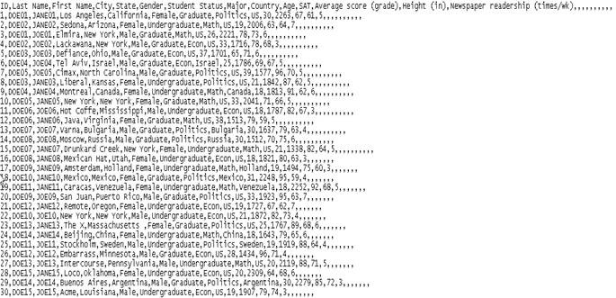
An example of *.CSV
(comma-separated-value) dataset
An example of tab separated dataset (can
have extension *.txt, *.dat, *.data, etc.)
An example of space separated dataset (*.prn,
*.txt)

An example of a text dataset (*.txt,
*.dat)

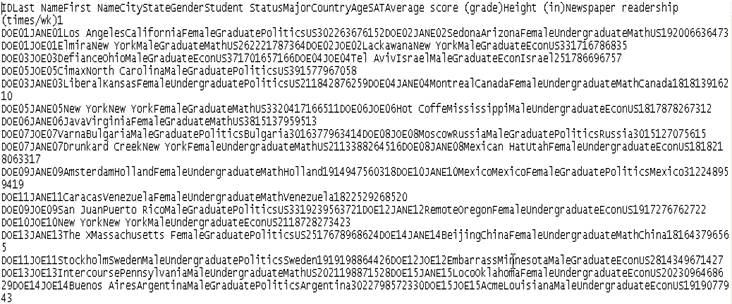
An example of plain text data (*.raw,
*.txt)
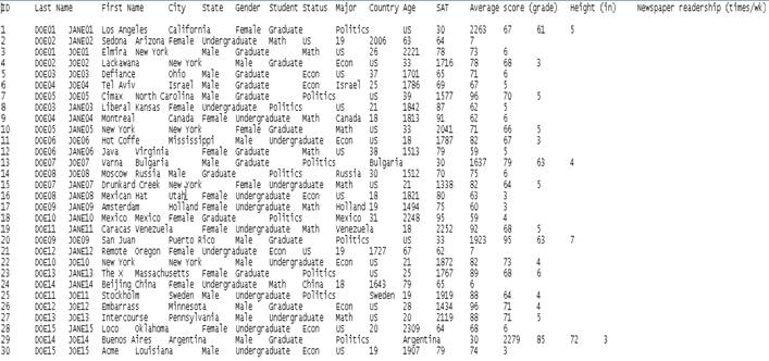
1.
Excel, spreadsheet format with extension
*.xls (Excel 2003 or earlier versions), *.xlsx (Excel 2007). Columns represent
variables, rows represent observations.

2.
Stata,
statistical software with extension *.dta. The extension of the file read ASCII
data is *.dct (dictionary file). Program files have extension *.do. Columns
represent variables, rows represent observations.
3.
SPSS,
statistical software with extension *.sav, *.por. Program files to read and to process data
have extension *.sps. Columns represent variables, rows represent observations.
4.
SAS,
statistical software with extension
*.sas7bcat, *.xpt. Program files have extension *.sas.
5.
MATLAB,
mathematical modeling and data analysis software with extension *.m
For a
comprehensive list of formats see:
http://whatis.techtarget.com/file-extension-list-M/0,289951,sid9,00.html
The trait
Numeric data
can have two different traits: qualitative or quantitative[4]
A qualitative
trait defines the categories that provide some meaning to the numerical value.
In reality this value is just a label. Data with some qualitative trait are
called categorical data. There are two types: nominal and ordinal.
Descriptive statistics for this type of data are in the form of percentages or
proportions. We find the type of data mostly (but not limited to) public
opinion, surveys or census data.
Here is an
example for this kind of data, in a recent New York Times article:
“A
study of nearly 4,000 men and women from
In
men, keeping quiet during a fight didn’t have any measurable effect on health.
But women who didn’t speak their minds in those fights were four times as
likely to die during the 10-year study period as women who always told their
husbands how they felt, according to the July report in Psychosomatic Medicine.
Whether the woman reported being in a happy marriage or an unhappy marriage
didn’t change her risk.”
[The
New York Times, Health section, web edition, October 2, 2007, link: http://www.nytimes.com/2007/10/02/health/02well.html?_r=1&oref=slogin]

Source:
The New York Times, Health section, web edition, October 2, 2007
http://graphics8.nytimes.com/images/2007/10/01/health/1002-sci-sub2WELL.gif
The
qualitative trait sex defines in
general two categories: females and males. These could be represented by the
numbers 1 (females) and 2 (males), or any other numbers or order. This type of
data is called nominal, in particular, binary since it has only
two categories.
Nominal data
can also be non-binary (more than two categories). Let’s say we are interested
in color preferences, so the qualitative trait is color. Here we could have more than two categories: black, white,
green, blue, red, etc. Which could be represented by the numbers 1, 2, 3, ,4,
etc.
For nominal
data numerical values are just a representation of the label without any actual
numerical property. In the color example, 2 is not necessarily greater than 1
nor is double than 1. Likewise, 1 is not lower than 1 nor is half of 2. No
arithmetic operation can be performed with this type of data. They are just
labels however this does not prevent them to be used for statistical analysis
(as binary or dummy variables).
For ordinal
data order matters. Examples: freshman, sophomore, junior, senior, etc; level
of agreement: strongly disagree, disagree, agree, strongly agree (this is known
as the Likert scale). You can label these responses as 1, 2, 3, 4, 5, etc. but
unlike nominal data order provides some meaning to the numbers: they go from
negative to positive, from low to high, from younger to older, from less
frequent to more frequent, or viceversa. Like nominal data the numbers just
represent labels without any numerical properties. There is no indication that
the difference between seniors and juniors is greater or lower than the
difference between juniors and sophomores. In the same way no arithmetic
operations can be performed here but there are some ways to use them for
complex statistical analysis.
A
quantitative trait produces numerical data from some sort of counting method or
measurement device. There are two types of numerical data: discrete and continuous.
Descriptive statistics for this type of data summarize location (i.e. the mean or average, median, mode) and variability (standard deviation,
variance, etc.)
Discrete data
is generally the result of some sort of counting, showing some gaps between
values. For example students, general population, number of cases, number of reports,
number of books cataloged, etc. In the image below, what do you see between
number 1 (ducky) and number 2 (bunny)? Well, you see nothing; there is some
empty space in between, there is a gap between number 1 number 2.
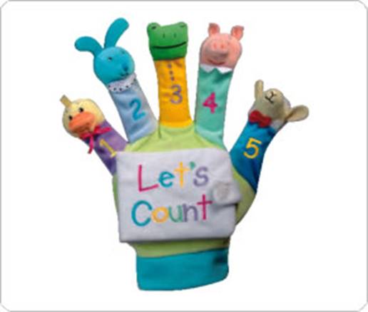
Continuous
data is generally the result of measurements. For example, same question, what
do you see between number 1 and 2? There is no empty space! No gap, there is
something in between, usually more numbers. So, with continuous data there is
always a value between any two, no gaps.
Examples are
time, height, distance, size, temperature, financial returns, etc.
In the same
way as categorical, continuous data have two groups: interval and ratio.
Interval data has a specific order and equal intervals (a $5 difference could
be from $1 and $6 or $10 and $15). Ratio in addition to be interval it has a
natural zero like income where 0 means “not money at all”. Temperature on the
other hand is only interval data since 0 indicates temperature and not the lack
of. In practice, the distinction between interval and ratio does not make much
of a difference.
When doing
data analysis, data taxonomy can be a problem and for some it is actually
irrelevant. Sometimes and in some cases categorical variables can be treated as
continuous when the sample size is large enough; continuous data can also be
converted to categorical and analyzed accordingly (like income brackets or age
categories). As homework read the following article and draw your own
conclusions.
http://www.spss.com/research/wilkinson/Publications/Stevens.pdf
Kachigan, Sam, Statistical analysis
: an interdisciplinary introduction to univariate & multivariate
methods.
Data levels
and measurement http://www2.chass.ncsu.edu/garson/PA765/datalevl.htm
Types of Data
http://www.stat.psu.edu/~resources/ClassNotes/ljs_04/sld018.htm
Introduction
to Categorical Analysis http://www.socialresearchmethods.net/tutorial/Cho/intro.htm
Categorical
data http://www.stat.yale.edu/Courses/1997-98/101/catdat.htm
Bloomberg
Financial Glossary http://www.bloomberg.com/invest/glossary/bfglosa.htm
Forbes
Financial Glossary http://www.forbes.com/tools/glossary/index.jhtml
Political
Glossary http://www.politicalglossary.net/
A Glossary of
Political Economy Terms http://www.auburn.edu/~johnspm/gloss/
Elections
Glossary http://www.pbs.org/elections/glossary/index.html
Glossary of
Social Science http://www.faculty.rsu.edu/~felwell/glossary/Index.htm